1.6T Optical Transceiver: 224G Signaling, High-Density PCB Design & Manufacturing Guide for Engineers and Buyers
Article Abstract
This engineering and procurement guide explains what a 1.6T Optical Transceiver is, why the shift from 112G to 224G-class electrical signaling transforms PCB design and manufacturing requirements, and how engineers and sourcing teams should select materials, stackups, fine-line processes and PCB suppliers. Written by a senior PCB manufacturing engineer with more than a decade of high-speed production experience, it covers mSAP, HDI microvia structures, copper roughness control, impedance validation and the biggest pain points in manufacturing high-density PCBs for 1.6T optical modules — with a practical qualification framework buyers can use immediately.
Author & E-E-A-T Statement
Senior Engineering Team, Shenzhen Hongda Circuit Technology Co., Ltd. (pcbkr.com). 10+ years in high-speed, HDI and fine-line PCB manufacturing for optical communication, AI server and data-center applications. Production floor data cited in this article reflects actual process capability, not marketing claims. Standards referenced: IEEE 802.3dj, IEEE 802.3ck, IPC-TM-650, IPC Class 3/3A, ISO 9001 / IATF 16949.
A 1.6T Optical Transceiver is a pluggable optical module that moves 1.6 terabits per second — twice the bandwidth of 800G — using eight 224G-class PAM4 electrical lanes defined under IEEE 802.3dj. It matters because AI training clusters and hyperscale data centers are consuming interconnect bandwidth faster than any previous generation. It creates new PCB challenges because 224G signaling makes the PCB itself part of the signal budget: insertion loss, copper roughness, via discontinuities, impedance tolerance and thermal density all become first-order design variables. This guide helps engineers design the board and helps buyers qualify the supplier.
What Is a 1.6T Optical Transceiver?
What Does “1.6T” Mean?
“1.6T” means 1.6 Tb/s of aggregate data rate. The industry reached it by doubling the electrical lane rate, not just adding lanes: 800G modules use 8 × 112G-class PAM4 lanes (IEEE 802.3ck), while 1.6T modules use 8 × 224G-class PAM4 lanes (IEEE 802.3dj) in form factors such as OSFP224 and OSFP-XD.
One point experienced engineers insist on: do not simplify “1.6T = 8 × 200G” into an absolute definition. Aggregate throughput, per-lane optical rate and electrical signaling rate are three different numbers that vary by architecture. What stays constant is the electrical channel requirement — 224G-class PAM4 with a Nyquist frequency above 50 GHz — and that is what lands on the PCB.
What Are the Main Components Inside a 1.6T Optical Transceiver?
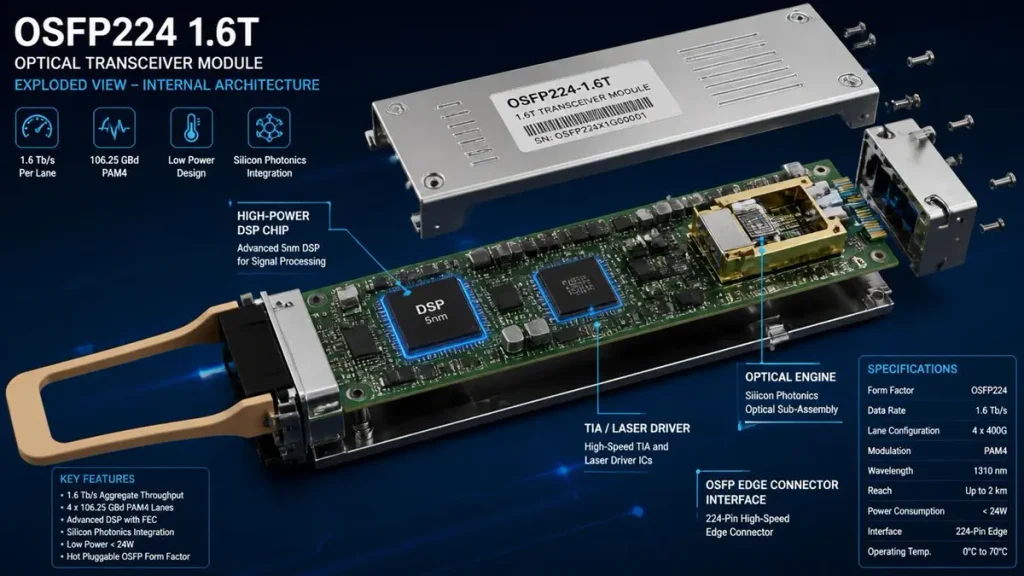
OSFP224 1.6T Optical Transceiver Internal Architecture & PCB Layout Diagram
- DSP (Digital Signal Processor) — the largest power consumer; performs PAM4 equalization, retiming and error correction
- TIA (Transimpedance Amplifier) and Laser Driver — analog front-end on the receive and transmit paths
- Optical Engine — silicon photonics or InP-based modulator/photodiode assembly
- Laser (EML, CW-DFB for silicon photonics, or VCSEL for SR8 variants) and Photodiode
- Electrical Interface — edge connector or board-to-board interface to the host switch card
- Optical Interface — MPO-16 dual-row or dual MPO-12 fiber connectors
Why Is 1.6T Different From Previous Optical Transceiver Generations?
1.6T is not simply “800G with more lanes.” At OFC 2026, the industry consensus was that 1.6T doubles bandwidth while simultaneously raising the bar on electrical channel loss, thermal management and manufacturing tolerance. Module power has climbed to roughly 40–45 W per OSFP224 port — about 3× an 800G module — which pushes heat directly into the PCB. Meanwhile the LPO (Linear Pluggable Optics) trend removes the DSP’s equalization from the module, which means the host PCB channel must be cleaner than ever, because there is less silicon left to fix a bad board.
How Does a 1.6T Optical Transceiver Compare With 800G?
| Parameter | 800G | 1.6T |
| Aggregate bandwidth | 800G | 1.6T |
| Electrical standard | IEEE 802.3ck | IEEE 802.3dj |
| Electrical signaling | 112G-class PAM4 | 224G-class PAM4 |
| Typical form factor | QSFP-DD / OSFP | OSFP224 / OSFP-XD |
| Module power draw | ~14–16 W | ~40–45 W |
| Signal integrity sensitivity | High | Very High |
| PCB loss sensitivity | High | Higher |
| Thermal challenge | High | Higher — liquid cooling at full density |
| Manufacturing tolerance | Tight | Tighter |
What Does 224G Mean for 1.6T?
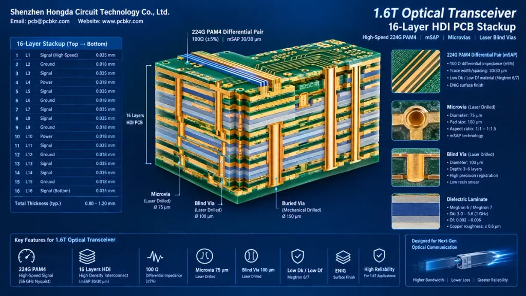
16-Layer High-Speed HDI PCB Cross-Section for 1.6T Optical Transceiver (224G PAM4 Signal Integrity Architecture)
224G-class PAM4 carries two bits per symbol at a 112 GBd baud rate. The Nyquist frequency exceeds 50 GHz, which means the PCB channel is now evaluated far into millimeter-wave territory. Key parameters: insertion loss (budgeted per channel, typically validated up to ~28–40 GHz+), return loss, crosstalk (NEXT/FEXT), skew, and equalization headroom — every dB of board loss consumes DSP or host SerDes margin.
The core engineering principle: at 224G-class signaling, the PCB is no longer a passive carrier. Its electrical channel characteristics become part of the system-level signal budget.
What Are the Main 1.6T Optical Transceiver Architectures?
1.6T DR8
Eight parallel 200G/lane optical fibers, single wavelength, silicon photonics or InP EML. Simplest optical design; common in AI cluster reach applications.
1.6T 2×FR4
Two 800G FR4 engines in one module — 4 wavelengths × 2 groups. Reuses mature 400G/800G optical technology; preferred for longer data-center interconnect reach.
OSFP224 and OSFP-XD
OSFP224 keeps the OSFP outline with 8 × 224G electrical lanes. OSFP-XD extends depth for future density. Both demand tighter connector-area routing and stricter thermal interfaces.
DSP-Based vs. Linear Optical Architectures
Full-DSP modules (40–45 W) equalize the channel internally. LPO modules remove the DSP, cutting power and latency but transferring the entire equalization burden to the host ASIC SerDes and the PCB channel. For PCB manufacturing, LPO is a stricter spec: lower loss, tighter impedance, cleaner vias.
Where Does CPO Fit Into the 1.6T Roadmap?
Co-packaged optics places optical engines beside the switch ASIC, shortening electrical paths dramatically. OFC 2026 showed CPO and pluggables coexisting — a hybrid roadmap. For PCB suppliers, CPO shifts demand toward substrate-like PCB (SLP) and advanced HDI with mSAP-class fine lines rather than conventional module boards.
What matters for this guide: each architecture changes the electrical channel length, thermal environment and manufacturing requirements — and therefore changes what you should specify in your RFQ.
Why Does 1.6T Create New High-Density PCB Engineering Challenges?
Signal Integrity
At 50+ GHz Nyquist frequencies, eye closure is driven by insertion loss, return loss, crosstalk, skew and reflections. A PAM4 eye has three eyes and much less vertical margin than NRZ; there is no room for sloppy channels.
Power Integrity
The DSP at 40+ W creates steep current transients. The PDN must keep voltage noise within spec across the whole module, driving decoupling capacitor placement, plane capacitance and — increasingly — embedded capacitor layers to replace discrete MLCCs at these densities.
Thermal Management
DSP, TIA and laser hotspots in a compact module are the number-one field failure trigger in optical module PCBs. Thermal vias, copper coin/heat-spreading planes, and thermal interface material selection must be designed together with the module mechanicals and airflow — never as an afterthought.
Mechanical and Routing Density
Compact modules with 0.35–0.4 mm fine-pitch BGAs, edge connectors and dense differential-pair routing push layer counts to 12–16+ layers and require HDI build-up structures.
The Biggest Pain Points in Manufacturing High-Density PCBs for 1.6T
1. Copper roughness inconsistency across lots. At 224G, conductor loss is dominated by skin-effect surface roughness. Suppliers quote HVLP copper but incoming foil varies lot to lot; without Rz measurement per lot, insertion loss wanders and SI validation results become irreproducible.
2. Microvia reliability in stacked structures. 1.6T modules commonly use stacked or staggered microvias with via-in-pad. Poorly controlled laser drilling and desmear leads to latent barrel cracks that pass electrical test and fail after thermal cycling in the field.
3. Impedance drift in volume production. The CAD says 100 Ω differential; production sees ±8–10% unless line width, dielectric thickness and Dk are statistically controlled panel by panel. This is the single most common dispute between design houses and fabs.
4. Layer-to-layer registration at fine pitch. Fine-pitch BGA escape routing at 20/20 μm line/space requires registration better than ±15 μm. Conventional subtractive lines cannot hold this; only LDI-imaged mSAP lines with disciplined process control can.
5. Thermal-mechanical warpage. Thin dielectrics + high layer counts + sequential lamination cycles = warpage that breaks assembly alignment. Managing warpage is a lamination engineering problem, not a fixturing problem.
6. Dk/Df data at the wrong frequency. Material datasheets quoting Df at 1 GHz are meaningless at 28–56 GHz. Requiring frequency-specific Dk/Df test data is essential, and many suppliers cannot provide it.
Why Does 224G Signaling Increase PCB Loss Sensitivity?
Insertion Loss and Return Loss
Loss scales with frequency and distance. Channel length, not module generation, should drive your loss budget — short-channel 1.6T designs can use mid-loss materials while long-channel designs genuinely need M8/M9-class laminates.
Dielectric Loss
Controlled by Df at operating frequency. Specify Df at 10 GHz, 28 GHz and 40 GHz minimum — not the 1 GHz headline number.
Conductor Loss and Copper Surface Roughness
At 224G, current flows in a skin depth of well under 1 μm. Rough copper behaves like a longer, lossier conductor. HVLP/VLP foils with Rz ≤ 2 μm are effectively mandatory on high-speed layers; standard HTE foil is not acceptable.
Via Discontinuities
Every via is an impedance discontinuity plus a potential stub resonator. Via count per channel, stub length and anti-pad geometry all consume loss budget. Where LPO is used, via budgets become critical because host-side equalization is limited.
Which PCB Materials Are Suitable for 1.6T Optical Transceivers?
Why Low-Loss Laminates Matter
Megtron 6, Megtron 7, Megtron 8 and M9-Class Materials
- Megtron 6 (M6) — proven at 112G; acceptable for short 224G channels
- Megtron 7 (M7) — mainstream choice for 224G module PCBs
- Megtron 8 / M9-class — for longer channels, CPO boards and the tightest loss budgets
How Should Engineers Compare Dk and Df?
Compare at identical test frequencies and methods (IPC-TM-650 2.5.5.x). Nominal values are marketing; frequency-swept data is engineering.
Why Dk/Df Alone Is Not Enough
Dk/Df does not capture copper roughness, resin content variation, glass weave skew (flat-glass spread-weave fabrics matter at 224G), or CAF resistance.
How Does Copper Roughness Affect Material Selection?
Material and foil must be selected as a system: a low-Df laminate with standard HTE foil underperforms a mid-loss laminate with HVLP foil at 224G.
When Is an Ultra-Low-Loss Material Actually Necessary?
The claim “every 1.6T PCB requires M8/M9” is false and expensive. The correct selection logic is:
Channel Length → Loss Budget → Frequency → Material → Copper → Stackup
A 30 mm breakout channel and a 120 mm host-card channel have fundamentally different material requirements. Buy material against your calculated loss budget, not against a competitor’s datasheet headline.
Does a 1.6T Optical Transceiver PCB Require mSAP?
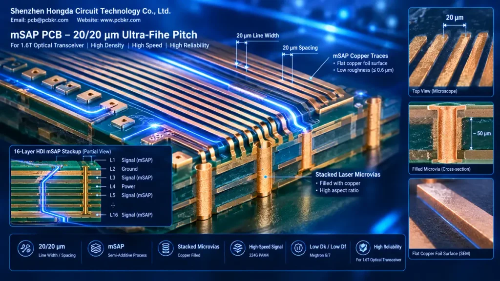
20/20 μm Ultra-Fine Pitch mSAP PCB Trace & Stacked Microvias for 1.6T Optical Transceiver
What Is mSAP?
Modified Semi-Additive Process: pattern-plate copper on a thin seed layer, then flash-etch the seed. Trace profiles are near-vertical with minimal undercut.
mSAP vs. Conventional Subtractive Etching
Subtractive etching with 18–35 μm foil realistically bottoms out around 50–75 μm line/space with trapezoidal profiles. mSAP reaches 20/20 μm in volume and 8/8 μm qualified for SLP builds, with ±5% impedance control versus ±10% typical for subtractive.
When Does a 1.6T Design Actually Need mSAP?
mSAP is an enabling technology, not an automatic requirement for every 1.6T design. If escape routing, line/space and impedance tolerances can be met on a subtractive line, use subtractive. If you need 20/20 μm or finer, near-vertical profiles for impedance consistency, or substrate-like density for CPO-adjacent designs, specify mSAP.
Hongda Circuit’s mSAP Capability (Latest Equipment & Technology)
At Shenzhen Hongda Circuit, our mSAP line has been in continuous production since 2024, with 2026 capacity targeting 20 μm/20 μm in volume and 8 μm/8 μm qualified for substrate-like PCB (SLP) builds. The line runs SCREEN Ledia LDI direct imaging (±1.5 μm registration) and a 3-in-1 horizontal plating line that improves throughput by 40% while reducing chemical consumption — the equipment directly determines whether fine-line capability is a datasheet claim or a shipped reality.
Does a 1.6T Optical Transceiver PCB Require HDI?
When Conventional Multilayer PCB Construction Is Enough
Short-channel, low-density module designs on 8–10 layers can remain conventional multilayer with through-holes and backdrilling.
When HDI Becomes Necessary
Fine-pitch BGA escape, 12–16+ layer counts, via-in-pad for shortest electrical paths — these force HDI build-up structures.
Microvias, Stacked and Staggered Microvias, Via-in-Pad, Blind and Buried Vias, Sequential Lamination
Backdrilling
Backdrill stubs on through-vias carrying 224G signals when stub resonance falls inside the channel band. If the signal transitions at an outer layer and the stub exceeds ~1/20 wavelength at Nyquist, backdrill.
| Design Requirement | Possible PCB Technology |
| High routing density | HDI |
| Fine-pitch BGA | Microvia |
| Short electrical path | Via-in-pad |
| Long through-via | Backdrilling |
| Fine-line routing | mSAP |
| High layer utilization | Sequential lamination |
How Should a 1.6T Optical Transceiver PCB Stackup Be Designed?
Signal and Reference Plane Arrangement
Every high-speed layer needs an adjacent unbroken reference plane. No exceptions at 224G.
Differential Pair Routing, Dielectric Thickness and Impedance Control
Tight coupling, symmetric geometry, and dielectric thickness chosen for manufacturability — not just electrical idealism. Thinner dielectrics are harder to laminate uniformly, and uniformity is impedance control.
Via Transitions and Return-Path Continuity
Stackup Symmetry and Lamination
A typical 12–16 layer example stackup (signal-ground-signal sandwich with build-up microvia layers on both sides) should be reviewed with your fabricator early. Note: example only — final layer count and stackup depend on channel length, routing density, module architecture and material selection.
What Impedance Control Is Required for 1.6T Optical Transceivers?
50 Ω Single-Ended vs. Differential Impedance
Most 1.6T channels are 100 Ω differential pairs; single-ended 50 Ω appears on control and power-adjacent signals.
Why 100 Ω Is Not Automatically 100 Ω in Production
Impedance is a statistical distribution, not a CAD number. Trace width ±5 μm, dielectric thickness ±10%, Dk variation, copper thickness, etch factor and registration all shift impedance. Specify ±5% or tighter with TDR coupon validation per panel, and require the actual distribution in the FA report — not a single “pass” number.
How Should PCB Manufacturers Validate Impedance?
TDR on impedance coupons, per-panel coupon placement, and stackup verification against the approved build. At Hongda Circuit, every high-speed job ships with TDR coupon data traceable to panel position.
How Does Copper Roughness Affect 1.6T PCB Performance?
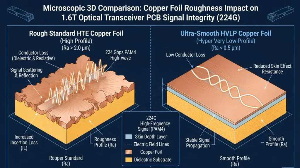
Microscopic 3D Comparison: Copper Foil Roughness Impact on 1.6T Optical Transceiver PCB Signal Integrity (224G)
Skin Effect, Conductor Loss and HVLP/VLP Copper
At 50+ GHz, skin depth approaches the scale of foil surface roughness. Rz becomes a first-order electrical parameter.
Why Standard Copper Specifications May Not Be Enough
“1 oz copper” says nothing about the surface. Procurement recommendation: do not specify copper foil only by thickness. Specify the electrical performance requirement (insertion loss at target frequency) and the relevant roughness parameters (Rz, treatment type) per lot.
How Do Via Structures Affect 1.6T Signal Integrity?
Via Stub, Backdrilling, Microvia, Via-in-Pad and Anti-Pad Design
Return Current Path
Every via transition must provide a continuous return path — a via changing reference layers without a return via nearby is a hidden reflector at 224G.
How Should Thermal Management Be Designed for 1.6T Optical Transceivers?
DSP Heat, Laser and TIA Heat, and Hotspots
Thermal Vias, Copper Planes, Heat Spreading, TIMs and Airflow
With 40–45 W per module, thermal design determines both optical performance (wavelength drift) and reliability. PCB thermal design must be evaluated together with module mechanical and airflow design — never treated as a separate PCB issue. LPO modules, with their tighter temperature sensitivity, punish boards with poor heat spreading.
What PCB Manufacturing Tolerances Matter for 1.6T Optical Transceivers?
| Manufacturing Parameter | Why It Matters |
| Line/space | Routing density |
| Layer registration | Differential-pair geometry |
| Dielectric thickness | Impedance |
| Copper thickness | Loss/current |
| Copper roughness | Conductor loss |
| Microvia diameter | HDI reliability |
| Via position | BGA/SI |
| Impedance tolerance | Signal integrity |
| Lamination | Reliability/warpage |
| Surface finish | Assembly (ENIG for fine pitch) |
How Should a 1.6T Optical Transceiver PCB Be Tested?
Fabrication Inspection
AOI, X-ray (microvia fill voids), microsection analysis, electrical testing.
Signal Integrity Testing
TDR for impedance and discontinuity mapping; VNA for insertion/return loss up to the channel’s highest significant frequency. Require S-parameter reports on coupons for 224G jobs.
Reliability Testing
Thermal cycling, reflow simulation, microvia reliability (IST or daisy-chain), CAF testing where applicable — per IPC Class 3 expectations.
Module-Level Validation
BER testing, eye diagrams, optical performance and thermal validation at the module OEM.
What Are the Most Common 1.6T Optical Transceiver PCB Design Mistakes?
1. Choosing materials based only on nominal Dk/Df
2. Ignoring copper roughness
3. Treating 100 Ω as an exact CAD number
4. Ignoring via stubs
5. Breaking return paths
6. Selecting the stackup too late
7. Assuming mSAP is always mandatory
8. Assuming HDI is always mandatory
9. Ignoring thermal coupling between DSP and laser
10. Selecting a PCB supplier after the design is frozen — the most expensive mistake on this list
How Should Buyers Qualify a 1.6T Optical Transceiver PCB Manufacturer?
Material Capability
Which low-loss laminates (M6/M7/M8/M9-class) can you process? Can you provide Dk/Df data at 10/28/40 GHz? What copper roughness options and per-lot Rz control do you offer?
Fine-Line and HDI Capability
mSAP line/space limits (volume vs. qualified), microvia diameter and stacking capability, via-in-pad plating, sequential lamination experience, registration data.
Signal Integrity Capability
In-house TDR and VNA, impedance coupon practice, SI engineering support during stackup review.
Quality and Reliability
IPC Class 3/3A, ISO 9001, IATF 16949, full lot traceability, reliability lab access.
Production Capability
Prototype → pilot → mass production scalability, capacity, lead time, yield management and statistical process control.
What Should Be Included in a 1.6T Optical Transceiver PCB RFQ?
- High-Speed Requirements: interface type, lane rate (224G PAM4), target impedance, insertion-loss target by frequency, channel length, differential-pair geometry rules.
- HDI Requirements: microvia structure (stacked/staggered), via-in-pad, backdrilling spec, sequential lamination cycles.
- Manufacturing Requirements: prototype quantity, production quantity, annual volume, qualification and testing requirements (TDR/VNA/S-parameter reports).
- Documentation: Gerber/ODB++, stackup drawing, drill files, impedance table, fabrication notes.
How Does a 1.6T Optical Transceiver PCB Move From Prototype to Mass Production?
Design → DFM → Prototype → SI Validation → Qualification → Pilot → Mass Production
When Should the PCB Manufacturer Be Involved?
Before the PCB layout is frozen. Stackup, material, via structure and tolerance decisions made after layout freeze are expensive rework — or silent field failures.
Why Choose Shenzhen Hongda Circuit for 1.6T Optical Transceiver PCB Manufacturing?
We present capability the way engineers evaluate it: Requirement → Capability → Evidence.
- High-speed PCB manufacturing: 112G/224G-class application experience with M6/M7/M8-class low-loss materials
- mSAP PCB manufacturing: 20/20 μm line/space in volume, 8/8 μm qualified for SLP, SCREEN Ledia LDI (±1.5 μm registration)
- HDI PCB manufacturing capability: microvia, sequential build-up, any-layer structures, via-in-pad with planarization
- Impedance-controlled PCB: ±5% with per-panel TDR coupons
- Inspection: 3D AOI, X-ray void inspection, flying-probe and fixture electrical test
- Quality: ISO 9001, IATF 16949, ISO 13485, AS9100D, IPC Class 3/3A
- Equipment: 3-in-1 horizontal plating line (+40% throughput, reduced chemical consumption), in-house TDR/VNA SI validation
Honest engineering statement: capability depends on the final stackup, material system, channel length, fabrication tolerances and customer specifications. Our engineering team evaluates these requirements during DFM and stackup review — we do not claim that every 1.6T PCB automatically meets 224G performance, and you should be skeptical of any supplier who does.
Ready to start? Request a PCB quote with your channel length, loss budget and layer count, and our engineering team will respond with a manufacturable stackup proposal. Email:pcb@pcbkr.com
Frequently Asked Questions About 1.6T Optical Transceivers and PCBs
What is a 1.6T Optical Transceiver and what does it mean for my PCB design?
A 1.6T Optical Transceiver is a pluggable module delivering 1.6 Tb/s using eight 224G-class PAM4 electrical lanes (IEEE 802.3dj). For your PCB, it means insertion loss budgets, 100 Ω differential impedance at ±5%, low-loss materials and copper roughness control are now design-critical rather than optional.
Does a 1.6T Optical Transceiver PCB require mSAP or HDI?
Not automatically. mSAP is needed when fine-line (≤20/20 μm) routing, near-vertical trace profiles or SLP-class density are required; HDI is needed for fine-pitch BGA escape and high routing density at 12+ layers. Evaluate against your channel length and routing density — a short-channel design may be conventional multilayer.
What is the difference between 1.6T DR8 and 2×FR4 architectures?
DR8 uses eight parallel 200G/lane single-wavelength fibers; 2×FR4 uses two 800G FR4 engines with four wavelengths each. Electrically both demand 224G-class channels, but DR8 modules tend toward silicon photonics integration with tighter thermal constraints on the PCB.
Which PCB materials are suitable for a 1.6T Optical Transceiver?
Megtron 6 for short channels, Megtron 7 as the mainstream 224G choice, Megtron 8/M9-class for long channels or LPO/CPO designs — always paired with HVLP copper (Rz ≤ 2 μm) and Dk/Df data specified at 10/28/40 GHz, not 1 GHz.
How should I qualify a 1.6T Optical Transceiver PCB manufacturer?
Verify low-loss material processing with frequency-specific Dk/Df data, mSAP/microvia capability with registration numbers, in-house TDR/VNA test capability, IPC Class 3 quality systems, and evidence of prototype-to-production yield management. Involve the manufacturer before layout freeze.
Is backdrilling necessary for 1.6T Optical Transceiver PCBs?
Backdrill when a through-via stub exceeds roughly 1/20 wavelength at the channel’s Nyquist frequency (~50+ GHz for 224G PAM4), or when stub resonance falls inside the channel band. If all high-speed transitions use microvias with no stub, backdrilling is unnecessary.
© 2026 Shenzhen Hongda Circuit Technology Co., Ltd. — www.pcbkr.com
About Author
David Chen LinkedIn Profile
David Chen is a Senior RF/PCB Process Engineer at Shenzhen Hongda Circuit Technology Co., Ltd., with over 12 years of experience in high-frequency PCB fabrication, impedance-controlled stack-up design, and Rogers/PTFE laminate processing. He also boasts an extensive professional background in PCBA manufacturing, PCBA testing, and PCBA optimization, with specialized expertise in high-precision PCBA fault analysis and rigorous PCBA reliability testing. The author has worked with high-layer-count server PCB fabrication, ultra-low-loss backplane stackups, and thermo-mechanical reliability optimization for AI infrastructure projects involving 112G and 224G PAM4 architectures. Skilled in complex circuit design and cutting-edge advanced PCB manufacturing processes, he delivers solutions that elevate product durability and performance across industrial applications. His technical articles focusing on PCBA manufacturing workflows and testing methodologies are widely cited by industry peers and technical platforms, and have gained attention and recognition from industry colleagues.